The Great Regression — with Python: Linear and Multilinear Regressions

For many real-life questions, we are interested in the relationship between two (or more) parameters. Typical questions are:

• What is the impact of more education on income?
• Does another cigarette hurt my health?
• How does the proximity to a factory affect my pollution exposure?

This article shows how to approach such questions using the simplest model. A model that assumes a linear relationship between the outcome (the thing that is affected) and the regressor(s) (the thing that affects the outcome).

Theoretical Discussions

This article has no theoretical purpose, but I want to introduce some notation. Of course, there are many more details that I won’t go into here.

Linear Regression

In the simplest regression, we model the (hidden) data generation process as linear. Therefore, we assume that the outcome (also called the response or dependent) and the regressors (also called the predictors or independent) have a linear relationship.

The prediction model looks like this:

The goal of linear regression is to minimize the residual sum of squares (RSS), which is the (squared) difference between the actual and predicted values.

This means that the linear algorithm chooses values for the coefficients that make our prediction as close to reality as possible.

Even though they assume a linear relationship, these models can get you a long way because in many cases they are a decent approximation for the (highly complex) real world.

Multilinear Regression

Multilinear regression follows the same logic by assuming a linear relationship between X and Y. However, instead of including only one regressor, we have multiple X’s (hence the name).

Data

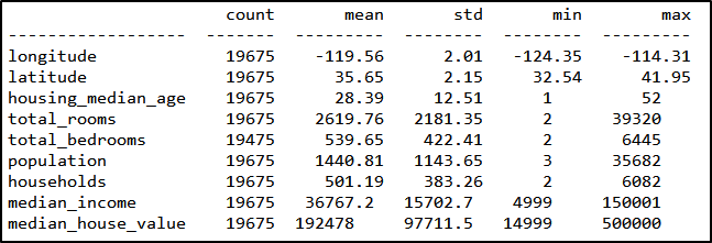
I am using the Kaggle data set on housing values in California. As you can see, the data contains several variables that define the median home value in a given area, including, for example, the median age of the house or the total number of rooms in a block.

Estimation

Linear Regression

In this example, I want to explain the house value by the median income within a block. So, the house value will be our dependent variable and the median income will be our predictor. After selecting our variables of interest, we split the data into training and test data and specify the model using sm.OLS(). I fit the model with robust standard errors (cov_type = “HC3”) because the assumption of homoscedasticity (constant variance of the error term) rarely holds in real-world examples.

# IN PYTHON:
#--------------------------------------------------
# specify test and training data

# defining our dependent and independent variable
y = housing_prep[["median_house_value"]]
x = housing_prep[["median_income"]]

# adding a constant such that it shows up in the regression
x = sm.add_constant(x)

# splitting into training and test data
x_train, x_test, y_train, y_test = train_test_split(
      x,
      y,
      test_size = 0.2,
      random_state = 0
)

#--------------------------------------------------
# run the linear regression model

# model specification
linear_model = sm.OLS(y_train, x_train)

# fitting the model
linear_model_fitted = linear_model.fit(cov_type = "HC3")

# print results
linear_model_fitted.summary()

# generate prediction
predicted_values = linear_model_fitted.predict(x_test)

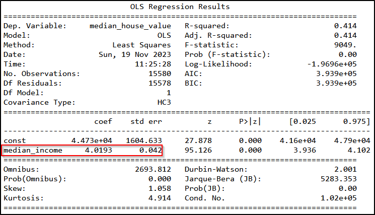
Printing the results shows that a higher median income is associated with higher house values within a given housing block. The effect is also highly statistically significant.

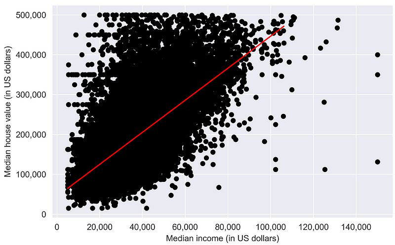
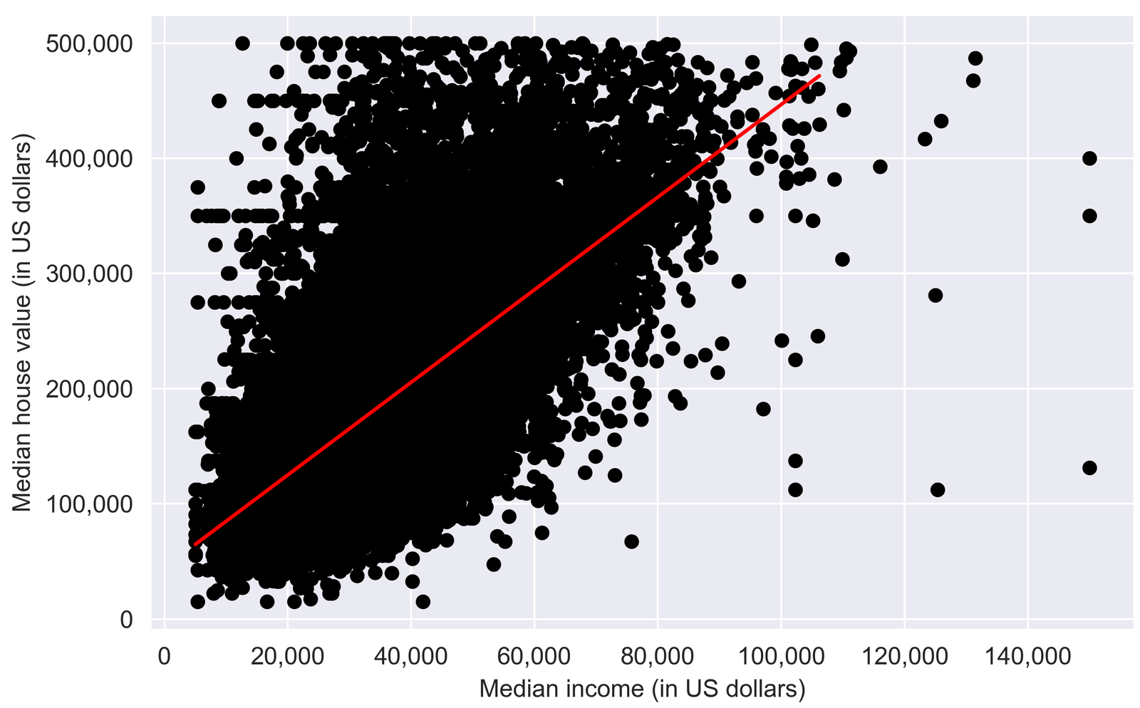
We can also plot the estimated relationship in a plot. The figure highlights the positive relationship between house values and income where the red fitted line (reflecting the estimated coefficient) has a clear upward slope.

Finally, to evaluate the fit of the model, let’s calculate the Root Mean Square Error. The RMSE reflects the average deviation between the predicted value and the actual value and can be used as a tool to judge the performance of the model.

# IN PYTHON:
#--------------------------------------------------
# Function for RMSE

def rmse(predicted_values, actual_values):
    return np.sqrt(((predicted_values - actual_values) ** 2).mean())

#--------------------------------------------------
# calculate RMSE
RMSE_linear_model = rmse(
    predicted_values = predicted_values,
    actual_values = y_test["median_house_value"].tolist()
)

The RMSE is quite large at 75,011.75. However, we are only controlling for one variable, which leaves room for improvement since there is a lot of noise left in the error term.

Multilinear Regression

To run the multilinear regression, we add more variables to the model, such as the number of rooms or the population. All of the included variables are highly statistically significant and the interpretation is the same as above.

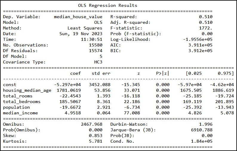
The RMSE for the multi-linear regression model is 67,754.97, which means that the more complex the model, the better the fit (for this example at least). However, including more variables, different functional forms, or even (regional) fixed effects could improve the fit even more.

Thank you for reading!

The code files can be found here. For those interested, you can also find an R-script in the folder generating similar outputs.

Check out my GitHub for other projects. You can also read the story on Medium. Feel free to reach out on LinkedIn.